The Big Sort

Without a Computer Science Degree, you’re most likely unfamiliar like I was with common engineering interview topics such as “Data Structures”, “Big O Notation” and “Sorting Algorithms”. After a five-hour crash course on AlgoExpert.io and after another five hours Googling sorting algorithms, I’ve written this post to summarize what I’ve learned into a quick read for other beginners.

Data Structures

Simply put, a data structure is a system for organizing data that can be stored, accessed and modified. There are all types of data structures (e.g. arrays, linked lists, hash tables), each with their own variable tradeoffs with storage, access and modification. These tradeoffs are the crux of application performance. The saying goes, you can’t optimized what you don’t measure. So, let’s understand how these tradeoffs in data structures are measured.

Time & Space Complexity

When it comes to determining the most performant data structure (or algorithm which we’ll get to later) to integrate into application development, it essentially comes down to optimizing two things - speed and memory. In engineering world, this is coined as Time & Space Complexity. I like to remember it as Time (speed) & Space (memory) Complexity (efficiency).

Big O Notation

Now that we understand what to measure, how do we measure it? The answer is a standardized measurement process intimidatingly referred to as Big O Notation. In short, Big O Notation measures the worst case scenario of Time & Space Complexity as the size of the input increases. I’ll try to further demystify this term by explaining the top four most common Big O Notation measurement results.

0(1) ie constant

As the input (eg into the Data Structure) increases, there is no increase in time complexity (ie it remains constant). This is the best Big O Notation.

O(n) ie linear

As the input increases, there is a linear (proportional) increase in time complexity. This is the third-best Big O Notation.

O(n^2) ie quadratic

As the input increases, there is a squared increase in time complexity. This is the worst Big O Notation.

O(log n) ie logarithmic

As the input increases, there is a logarithmic increase in time complexity. This is the second-best Big O Notation…but whoa - what does logarithmic mean?!

Logarithmic

Time to get mathematical. Remember that space is memory and time is speed. Memory relates to inputs as speed relates to operations. Let’s think of those two numbers (inputs & operations) as a ratio.

O(log n) is very efficient as the ratio of the number of operations to the number of inputs decreases as n increases. Each subsequent operation cuts the input in half. As the inverse of a logarithmic function is an exponential function, we can also think of it as one extra operation doubles the input.

In formula form, 2^x = log n. In written form, two to the power/exponent of x equals log n. Let’s remember that the power/exponent increases little compared to n. For example and roughly speaking, 2^20 = 1M whereas 2^30 = 1B.

Sorting Algorithms

Now that we have a general understanding of Data Structures and Big O Notation, let’s apply those concepts to Sorting Algorithms. I glossed over the space (memory) variability of various Data Structures in order to focus on the most relevant variable of time (speed) complexity for Data Structures to more simply understand Big O Notation.

However, it’s important to note that to evaluate Big O Notation with Sorting Algorithms, there is an equal importance placed on both the variability of space complexity AND time complexity.

For Sorting Algorithms, I’ll skip over the details of their Big O Notation evaluations. That’s a post for another day. Instead, I will give us instant gratification with my summaries of the most popular Sorting Algorithms along with their respective visual representations through animations from Wikipedia.

Bubble Sort

method: compares every adjacent element to ‘bubble’ max
advantages: stable (objects with the same keys maintain the same order in the sorted output as in the unsorted input), simplicity
complexity: O(n^2) Time / 0(1) Space

Insertion Sort

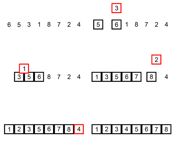
method: compares next element with every element and ‘inserts’ appropriately
advantages: stable, good for partially sorted arrays
complexity: O(n^2) Time / O(1) Space

Selection Sort

method: finds smallest element then repeatedly ‘selects’ and swaps the next-smallest element
disadvantage: unstable
complexity: O(n^2) Time / O(1) Space

Quick Sort

method: repeatedly divide and conquer elements into three parts (<, middle, >)
disadvantage: unstable
complexity: O(n^2) Time / O(log n) Space

Merge Sort

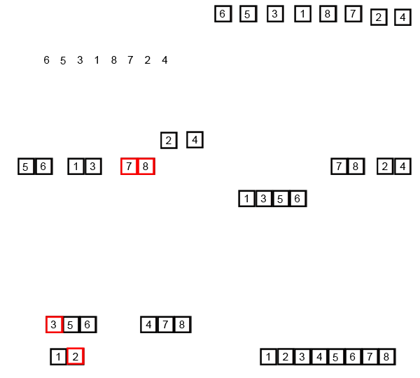
method: divide and conquer elements into equal parts to compare (left-most / index 0) by recursive merges
advantages: stable, best for sorting Linked Lists
disadvantage: worst for partially sorted arrays
complexity: O(log n) Time / 0(n) Space

Heap Sort

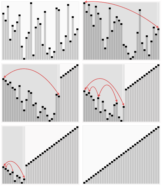
method: creating heap then repeatedly replacing largest and smallest elements into an array
advantage: fastest
disadvantage: unstable
complexity: O(log n) Time / 0(1) Space